Korelasi dan Regresi

KORELASI DAN REGRESI LINEAR SEDERHANA

1.      Korelasi

Pada semua kejadian, baik kejadian ekonomi maupun lainnya, pasti ada faktor yang menyebabkan terjadinya kejadian-kejadian tersebut. Misal, angka penjualan suatu barang yang turun disebabkan oleh naiknya harga barang tersebut. Contoh lain, seorang anak yang tidak belajar mendapatkan nilai jelek pada saat ulangan, dll.

Uraian di atas menunjukkan adanya hubungan atau korelasi antara kejadian yang satu dengan kejadian yang lainnya. Kejadian itu dapat dinyatakan dengan perubahan nilai variabel. Misal, jika x merupakan variabel harga, maka naik turunnya harga dapat dinyatakan dengan perubahan nilai x. Dan apabila y merupakan variabel hasil penjualan, maka naik turunnya hasil penjualan dapat dinyatakan dengan perubahan nilai y. Jadi, hubungan antara dua kejadian dapat dinyatakan dengan hubungan dua variabel x dan y. Disini saya hanya akan menjelaskan tentang hubungn antara dua variabel, hubungan linier lebih dari dua variabel akan dijelaskan pada subbab berikutnya.

Pada contoh diuraian sebelumnya, kita tentu setuju jika dikatakan bahwa naik turunnya harga mempengaruhi hasil penjualan. Namun dalam hal ini kita tidak tahu pasti seberapa besar pengaruhnya. Analisis korelasi yang akan dibahas kali ini berfungsi untuk mengetahui seberapa besar atau seberapa kuat suatu relasi antar dua variabel.

2.      Ukuran korelasi

            Hubungan dua variabel ada yang positif dan negatif. Suatu hubungan dikatakan positif apabila kenaikan/penurunan x pada umumnya diikuti oleh kenaikan/penurunan y. Sebaliknya dikatakan negatif bila kenaikan/penurunan x pada umumnya diikuti oleh penurunan/kenaikan y.  Perhatikan Gambar 1 dan 2.

Gambar 1. Korelasi positif

Gambar 2. Korelasi negatif.

Contoh korelasi positif:

            x = pupuk,                   y = produksi

            x = biaya iklan,            y = hasil penjualan

            x = berat badan,          y = tekanan darah

Contoh korelasi negatif:

            x = harga suatu barang,           y = permintaan barang

            x = pendapatan masyarakat,   y = kejahatan ekonomi

Apabila diagram pencar tidak teratur, artinya kenaikan/penurunan x tidak berpengaruh pada kenaikan/penurunan x. Maka dapat dikatakan x dan y tidak berkorelasi.

3.      Koefisien korelasi

            Kuat dan tidaknya hubungan antara x dan y apabila dinyatakan denagn fungsi linier, diukur dengan suatu nilai yang disebut koefisien korelasi (r). Nilai koefisien korelasi ini paling sedikit bernilai -1 dan paling besar bernilai 1. Jadi dapat dinyatakan sebagai berikut:

-1<= r >= 1

Artinya:

·         Jika r = 1, hubungan x dan y sempurna dan positif (mendekati 1, yaitu hubungan sangat kuat dan positif).

·         Jika r = -1, hubungan x dan y sempurna dan negatif (mendekati -1, yaitu hubungan sangat kuat dan negatif).

·         Jika r = 0, tidak ada hubungan atau lemah sekali hubungan antara x dan y.

Cara menghitung nilai r yakni:

Rumus ini merupakan rumusan koefisien korelasi Pearson.

4.      Koefisien Penentu

            Nilai x dikatakan mempengaruhi y karena kenaikan atau penurunan x mempengaruhi nilai y. Namun dalam diagram pencar, nilai y memiliki nilai yang bervariasi meskipun nilai y naik dalam deret ukur. Hal ini terjadi karena nilai y tidak hanya dipengaruhi oleh variabel x namun juga beberapa faktor lain. Misal, hasil penjualan tidak hanya dipengaruhi oleh harga pasar tapi melainkan juga dipengaruhi oleh pendapatan masyarakat, selera, dll. Dari sini timbul pertanyaan, beraa besarnya kontribusi dari x terhadap naik turunnya nilai y? Untuk menjawab pertanyaan ini harus dihitung dulu suatu koefisien yang disebut keofisien determinasi atau koefisien penentu (KP). Nilai KP dicari dengan rumus,

KP = r²

Jika r = 0.9 maka nilai KP = (0.9)² = 0.81 atau 81%. Hal ini berarti besar kontribusi dari x terhadap nilai y sebesar 81%, dan 19% lainnya adalah kontribusi dari faktor-faktor lainnya.

Contoh soal korelasi:

1. Jika x adalah presentase kenaikan biaya iklan dan y adalah presentase kenaikan hasil penjualan, kemudian berdasarkan tabel dibawah ini, hitunglah koefisien korelasi (r)!

x	1	2	4	5	7	9	10	12
Y	2	4	5	7	8	10	12	14

Penyelesaian :

untuk menghitung r diperlukan lembaran kerja yang disusun berdasarkan rumus sebagai berikut :

x	Y	x2	y2	xy
1	2	1	4	2
2	4	4	16	8
4	5	16	25	20
5	7	25	49	35
7	8	49	64	56
9	10	81	100	90
10	12	100	144	120
12	14	144	196	168
Σxi = 50	Σyi = 62	Σxi2 = 420	Σyi2 = 598	Σxiyi = 499

2.  2. Jika X adalah presentase kenaikan harga dan Y adalah presentase kenaikan hasil penjualan, kemudian berdasarkan tabel dibawah ini, hitunglah koefisien korelasi (r) dan kofisien determinasi (KP) !

X	2	4	5	6	8	10	11	13	14	15
Y	15	14	12	10	9	8	6	4	3	2

Penyelesaian :

untuk menghitung r diperlukan lembaran kerja yang disusun berdasarkan rumus sebagai berikut :

X	Y	X2	Y2	XY
2	15	4	225	30
4	14	16	196	56
5	12	25	144	60
6	10	36	100	60
8	9	64	81	72
10	8	100	64	80
11	6	121	36	66
13	4	169	16	52
14	3	196	9	42
15	2	225	4	30
ΣXi=88	ΣYi=83	ΣXi2= 956	ΣYi2=875	ΣXiYi=548

Kesimpulan: hubungan X dan Y kuat dan negatif. Dengan demikian, nilai KP = r² = (-0.99)² = 0.9801 = 0.98 = 98%.

5.      Regresi

Apa perlunya mengetahui hubungan antar variable? Di dalam perencanaan, selain data masa lampau dan masa sekarang, juga diperlukan data hasil ramalan yang menggambarkan kemampuan di masa yang akan datang. Misalnya, perusahaan dalam merencanakanproduksi memerlukan ramalan hasil penjualan (kemampuan menjual di masa yang akan datang, sehingga dapat dicegah terjadinya overproduction atau underproduction).

Apabila dua variable X dan Y mempunyai hubungan, maka nilai variable X yang sudah diketahui dapat digunakan untuk menaksir/memperkirakan nilai variable Y.

Variable Y yang nilainya akan diramalkan disebut variable tidak bebas (dependent variable), sedangkan variable X yang nilainya digunakan untuk  meramalkan nilai Y disebut variable bebas (independent variable).

Jadi analisis korelasi membantu kita untuk mengetahui seberapa kuat hubungan antara dua variable, sedangkan analisis regresi membantu kita untuk:

1.      Mengetahui apakah ada relasi/hubungan antar variable

2.      Membantu menentukan jenis persamaan yang akan digunakan untuk menentukan hubungan tersebut..

        

6. Diagram pencar

         Jika terdapat sebuah data antara dua variable dan kita belum dapat memastikan apakah data tersebut memiliki hubungan satu sama lain atau tidak, cara untuk mengetahuinya adalah dengan cara menggunakan diagram pencar (scatter diagram).

Gambar 3. Macam-macam scatter diagram

         Pada kesempatan ini hanya akan dijelaskan mengenai regresi linear sederhana yakni regresi yang berbentuk garis lurus atau linear (gambar (a), dan (b)).

7. Persamaan Regresi Linear Sederhana

         Bentuk umum persamaan regresi linier:  y = a + bx

                        y          : peubah takbebas                    x          : peubah bebas

                        a          : konstanta                               b          : kemiringan/gradien

                                               

·      Penetapan Persamaan Regresi Linier Sederhana

Dengan,           n  : banyak pasangan data

y_i  : nilai peubah takbebas y ke-i

x_i  : nilai peubah bebas x ke-i

Contoh soal regresi linear sederhana:

1.      Berikut adalah data Biaya Promosi dan Volume Penjualan  PT BIMOIL perusahaan Minyak Goreng. Banyaknya data ada lima data. Tentukan persamaan regresinya!

Tahun	x Biaya Promosi (Juta Rupiah)	Y Volume Penjualan (Ratusan Juta Liter)	xy	x²	y²
1992	2	5	10	4	25
1993	4	6	24	16	36
1994	5	8	40	25	64
1995	7	10	70	49	100
1996	8	11	88	64	121
S	Sx = 26	Sy = 40	Sxy = 232	Sx² =158	Sy² = 346

bentuk umum persaman regresi linier sederhana : y = a + b x

y = a + b x       ®        y = 2.530 + 1.053 x

2.      Diketahui hubungan Biaya Promosi  (x dalam Juta Rupiah) dan y (Volume penjualan dalam Ratusan  Juta liter) dapat dinyatakan dalam persamaan regresi linier berikut

y = 2.530  + 1.053 x. Perkirakan Volume penjualan jika dikeluarkan biaya promosi Rp. 10 juta ?

Penyelesaian:   y = 2.530  + 1.053 x

                        x = 10

                        y = 2.53 + 1.053 (10) = 2.53 + 10.53 = 13.06 (ratusan juta liter)

Volume penjualan = 13.06 x 100 000 000 liter

8. Standar Error Estimasi

         Dalam menggunakan persamaan regresi untuk melakukan suatu perkiraan, terdapat satu pertanyaan penting mengenai seberapa kuat hubungan antar variable bebas dan terikatnya; atau dengan kata lain, seberapa besar derajat ketergantungannya (dependability) hasil perkiraan tersebut. Hal ini dapat lebih dimengerti dengan memperhatikan gambar 4 (a), terlihat bahwa titik-titik data terpencar lebih rapat di sekitar garis regresi dibandingkan dengan titik-titik data pada gambar 4 (b). Dengan nalar secara awam saja, kita dapat mengatakan bahwa suatu estimasi yang dilakukan dengan persamaan garis regresi untuk keadaan pada gambar 4 (a) akan lebih baik dibandingkan untuk keadaan pada gambar 4 (b).

Gambar 4

            Ukuran yang mengindifikasi derajat variasi sebaran data di sekitar garis regresi dapat menunjukkan seberapa besar derajat keterikatan perkiraan yang diperoleh dengan menggunakan persamaan regresi tersebut. Ukuran ini dinamakan sebagai standar error estimasi. Dalam definisi yang lebih tepat standar error estimasi estimasi (s_y,x) adalah deviasi standar yang memberikan ukuran penyebaran nilai-nilai yang teramati di sekitar garis regresi, dirumuskan sebagai berikut:

Contoh soal:

Dari suatu praktikum fisika dasar diperoleh data yang menghubungkan variabel bebas x dan variabel terikat y seperti ditunjukkan dalam tabel berikut:

Ujian ke-	x	y
1	6	30
2	9	49
3	3	18
4	8	42
5	7	39
6	5	25
7	8	41
8	10	52
S	56	296

Jika diasumsikan memiliki bentuk hubungan yang linear, maka hitunglah persamaan garis regresinya dan standar error estimasinya!

Penyelesaian:

Ujian ke-	x	y	xy	x2	y2
1	6	30	180	36	900
2	9	49	441	81	2401
3	3	18	54	9	324
4	8	42	336	64	1764
5	7	39	273	49	1521
6	5	25	125	25	625
7	8	41	328	64	1681
8	10	52	520	100	2704
S	56	296	2257	428	12920

·         Nilai konstanta b dapat ditentukan:

·         Nilai konstanta a dapat ditentukan:

Jadi persamaan regresi linear yang menggambarkan hubungan antara variabel x dan y dari data sampel pada percobaan/praktikum di atas adalah:

y = 1.0277 + 5.138 x

·         Menghitung standar error estimasi:

Perkiraan atau Pendugaan Interval

Pada teori pendugaan (estimation theory) terdapat dua hal yang penting yaitu pendugaan interval (confidence interval, atau interval estimation) dan pendugaan tunggal (prediction interval atau point estimation). Pendugaan interval dimaksudkan untuk menggambarkan nilai tengah untuk setiap nilai X tertentu, sedang pendugaan tunggal untuk menggambarkan kisaran nilai untuk setiap nilai X tertentu.

1.1  Pendugaan Nilai – Tengah Y.

Pendugaan interval nilai tengah Y dimaksudkan untuk mengetahui nilai dugaan bagi Y untuk seluruh nilai X yang diketahui. Telah disinggung pada sub-bab sebelumnya bahwa dalam model regresi linier ini, dengan adanya nilai pengamatan dari nilai dugaannya, suatu nilai peubah bebas X tertentu dapat memberikan beragam nilai peubah Y yang bervariasi  yang pusatnya diperkirakan terletak pada titik y_x = β₀ + β₁x.  Dengan kata lain, nilai harapan Y pada X tertentu adalah β₀ + β₁X. Nilai tengah Y tersebut diduga oleh y = b₀ + b₁x dengan galat baku:

sehingga selang kepercayaan (1 – α) 100% bagi µ_yıx adalah:

Contoh 1

Berikut ini adalah delapan pengukuran pada tinggi anak dengan tinggi bapak dan tinggi anak sulungnya (cm). 

Tentukan selang kepercayaan 95% bagi nilai-tengah tinggi badan anak yang bapaknya memiliki tinggi 165 cm!

Jawab:

Untuk pengamatan tersebut dapat dibuat tabel berikut ini (X untuk tinggi bapak, Y untuk tinggi anak)

Model Regresinya adalah:

sehingga Y = 64.70 + 0.623x

Penduga titik nilai – tengah tinggi anak yang bapaknya memiliki tinggi 165 cm adalah:

 µ_y|x=165 = 64.70 + (0.623) (165) = 167.495 cm

Galat baku dugaan tersebut adalah:

dengan t_0.025,6 = 2.447

Selang kepercayaan 95% tinggi anak yang bapaknya memiliki tinggi 165 cm adalah :

  

1.2. Pendugaan Satu Nilai y pada x tertentu (Pendugaan Tunggal)

           

Nilai y pada x tertentu juga diduga dengan y = b₀ + b₁x. Berbeda dengan nilai tengahnya, galat baku pendugaan satu nilai y adalah

 sehingga selang kepercayaan (1 - α) 100% bagi y pada x tertentu adalah

Contoh 2

Untuk data pada contoh 1 tentukan selang kepercayaan 95% bagi tinggi badan seorang anak yang bapaknya memiliki tinggi 165 cm!

Jawab:

Penduga titik nilai y pada tinggi anak yang bapaknya memiliki tinggi 165 cm adalah

y_|x=165 = 64.70 + (0.623) (165) = 167.495 cm

Galat baku dugaan tersebut adalah:

dengan t_0.025,6 = 2.447

Selang kepercayaan 95% tinggi anak yang bapaknya memiliki tinggi 165 cm adalah :

 

  Tabel Analisis Ragam

                        Analisis ragam atau analysis of variance(ANOVA) adalah suatu metode untuk

menguraikan keragaman total data menjadi komponen-komponen yang mengukur

berbagai sumber keragaman. Pengujian model dapat juga dilakukan dengan menggunakan analisis ragam. Perhatikan bahwa jumlah kuadrat total dapat diuraikan menjadi jumlah kuadrat regresi dan jumlah kuadrat galat sebagai berikut:

Sementara itu, derajat bebas masing – masing jumlah kuadrat tersebut berturut – turut adalah:

DB(Total) = n – 1

DB(Regresi) = 1

DB(Galat)= n-2

Sedangkan DB(Total)= DB(Regresi) + DB(Galat)

Tabel Analisis dengan demikian dapat disusun, sebagai berikut:

Nilai F_hitung dari table analisis raga mini adalah nilai F uji atas hipotesis H₀ : σ²_regresi = σ²_sisa  v.s. H₁ : σ²_regresi = σ²_sisa

Nilai F_hitung yang lebih dari F_{α, DB(Regresi),DB(Galat)} yang berarti tertolaknya H₀ pada taraf nyata α, diinterpretasikan bahwa persamaan regresi linear yang terpasang pada data adalah berperan dalam menjelaskan keragaman total. Dengan kata lain, tertolaknya H₀ dalam uji-F tadi menunjukkan adanya peran peubah bebas dalam menjelaskan keragaman peubah tak bebas, atau keragaman data bukanlah sekedar keragaman acak tetapi berkaitan dengan keragaman peubah bebas menurut persamaan regresi linier.

Contoh 3

Untuk data pada contoh 1 buatlah tabel analisis ragam untuk regresi tinggi badan anak pada tinggi badan bapaknya!

Jawab :

Untuk data pada contoh 1 dapat disusun tabel perhitungan sebagai berikut :

Dari tabel diperoleh:

            JK (Galat)       =  375.80

JK (Total)        =  463.50

JK (Regresi)    = JK(Total) – JK (Galat)

= 463.50 – 375.80

= 87.7

Tabel Analisis Ragam untuk regresi tinggi badan anak pada tinggi badan bapaknya :

Adapun F_0.05,1.6 = 5.99

Dengan F_hitung tidak lebih dari F_0.05,1.6 maka keputusan ujinya adalah tidak tolak H₀. Berdasarkan data tabel tersebut , persamaan regresi linier yang terpasang pada data belum bisa dikatakan berperan dalam menjelaskan keragaman total.

        Kesesuaian Model Regresi

Kesesuaian model merupakan ukuran untuk mengetahui kesesuain atau ketepatan antara nilai dugaan atau garis regresi dengan data sample. Ukuran kesesuaian  model ini disebut Koefisien Determinasi (R²).  Koefisien Determinasi adalah bagian dari keragaman total variable tak bebas Y (variable yang dipengaruhi atau dependent) yang dapat diterangkan atau diperhitungkan oleh keragaman variable bebas X (variabel yang mempengaruhi atau independent). Jadi koefisien determinasi adalah kemampuan variable X (variable independent) mempengaruhi variable Y (variable dependent). Semakin besar koefisien determinasi menunjukan semakin baik kemampuan X menerangkan Y. Besarnya koefisien determinasi adalah kuadrat dari koefisien korelasi dan dirumuskan sbb :

Nisbah kuadrat tengah total pada kuadrat tengah galat menunjukkan besarnya keragaman data yang tidak terjelaskan oleh model. Koefisien determinasi dengan demikian menyatakan besarnya keragaman yang terjelaskan oleh model. Nilai minimum koefisien determinasi adalah 0, dan nilai maksimumnya adalah 1. Semakin besar nilai koefisien determinasi, mendekati angka 1, semakin sesuai model yang dipasang dengan data yang dibicarakan. Koefisien determinasi kadang – kadang juga dinyatakan dalam persen, sehingga nilainya berkisar antara 0 – 100%.

Contoh 4

Hitunglah besarnya koefisien determinasi untuk regresi tinggi badan anak pada tinggi badan bapaknya!

Jawab:

Dari contoh 1, koefisien determinasi regressi tersebut adalah:

Koefisien determinasi untuk model regresi ini sangat kecil, menunjukkan model ini kurang baik dalam menjelaskan keragaman peubah respon dalam kaitannya dengan peubah penjelas. Kurang baiknya model ini mungkin karena antara kedua peubah tersebut pada kenyataannya tidak berkaitan satu sama lain, atau keterkaitan antara peubah tersebut ada tetapi tidak linier.

 

REGRESI GANDA

I.      Pengertian Regresi Ganda

Regresi ganda adalah regresi suatu variable terikat yang memiliki  lebih dari satu variable bebas. Bentuk persamaan umum dari regresi ganda adalah :

Regresi ganda berguna untuk mencari pengaruh dua variable predictor atau untuk mencari hubungan fungsional dua variable penjelas (variable bebas) atau lebih terhadap variable respon(variable terikat). Penyelesaian regresi ganda dapat menggunakan notasi matriks dan persamaan linear dengan metode substitusi dan eliminasi.

II.         Metode Regresi Ganda

a.     Metode Matriks

Dalam notasi matriks, p merupakan variable bebas berdasarkan jumlah pengamatan (n):

Dengan

Y = vector variable terikat berukuran nX1

X = matriks variable bebas berukuran n X (p+1)

 beta   = vector koefisien regresi berukuran (p+1) X 1

 

Pendugaan koefisien regresi di buat dengan cara mendapatkan solusi atas persamaan normal yaitu

Sehingga

Selanjutnya ragan bagi  beta  , s²{b}, dalam notasi matriks dituliskan sebagai :

dengan

Sehingga uji hpotesis atas H0 : b_k ¹ 0 ; k = 0, 1, 2, 3, …….., p

Dapat di buat dengan criteria uji T.  Tolak H0 jika t  lebih kecil atau sama dengan -t_a/2,n-(p+1) atau sama dengan -t_a/2,n-p dengan       t = be / s{bk}  , P(T ³ -t_a/2,n-(p+1)) = a/2, dan  

Pendugaan Nilai Peubah Respon galat baku bagi dugaan nilai-tengah Y dan dugaan nilai Y pada X tertentu, X_t’ dalam bentuk matriks masing-masing adalah :

Selang kepercayaan (1-a) 100% bagi nilai tengah Y dan dugaan nilai Y pada X tertentu , Xt'  masing-masing adalah:

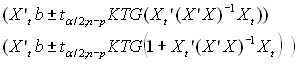
Jumlah kuadrat total, jumlah kuadrat regresi dan jumlah kuadrat galat dalam matriks ditulis masing-masing sebagai berikut:

Derajat bebas yang berpadanan dengan masing-masing jumlah kuadrat tersebut adalah :

Koefisien determinasi yang merupakan ukuran kesesuaian model dapat dihitung yaitu:

 

a.     Metode Persamaan Linear

Persamaan regresi ganda dapat digunakan dalam perhitungan nilai Y untuk setiap perhitungan nilai X₁dan X₂. Perubahan nilai Y disebabkan oleh perubahan X₁, ketika X₂ konstan ataupun sebaliknya. Data pada table regresi, yang terdiri dari variable X₁, X₂, dan Y dapat di hitung dengan persamaan sebagai berikut:

 Persamaan regresi ganda dapat di uji dengan persamaan berikut ini:

Kemudian mencari R_hintung dengan rumus:

Setelah R_hintung  diperoleh maka kuadratkanlah R_hintung. Kemudian menghitung F _{sign hitung} dengan rumus:

Contoh soal:

1.     Diberikan data sebagai berikut:

Y	X1	X2
23.3	5	13
24.5	6	14
27.2	8	17
27.1	9	17
24.1	7	14
23.4	5	13
24.3	6	14
24.1	7	14
27.2	9	17
27.3	8	17
27.4	8	17
27.3	9	17
24.3	6	14
23.4	5	13
24.1	7	14
27	9	17
23.5	5	13
24.3	6	14
27.3	8	17
23.7	7	14

Tentukan koefisien regresi X₁, X₂, dan Y dengan metode:

i)       Persamaan linear

hitung pula nilai determinasi korelasiberganda dan F _{sign hitung}

ii)    Matriks

Penyelesaian:

Koefisien regresi X₁, X₂, dan Y

i)          Persamaan linear

Buat table sebagai berikut:       

No	Y	X1	X2	X1Y	X2Y	X1X2	(X1)2	(X2)2	Y2
1	23.3	5	13	116.5	302.9	65	25	169	542.89
2	24.5	6	14	147	343	84	36	196	600.25
3	27.2	8	17	217.6	462.4	136	64	289	739.84
4	27.1	9	17	243.9	460.7	153	81	289	734.41
5	24.1	7	14	168.7	337.4	98	49	196	580.81
6	23.4	5	13	117	304.2	65	25	169	547.56
7	24.3	6	14	145.8	340.2	84	36	196	590.49
8	24.1	7	14	168.7	337.4	98	49	196	580.81
9	27.2	9	17	244.8	462.4	153	81	289	739.84
10	27.3	8	17	218.4	464.1	136	64	289	745.29
11	27.4	8	17	219.2	465.8	136	64	289	750.76
12	27.3	9	17	245.7	464.1	153	81	289	745.29
13	24.3	6	14	145.8	340.2	84	36	196	590.49
14	23.4	5	13	117	304.2	65	25	169	547.56
15	24.1	7	14	168.7	337.4	98	49	196	580.81
16	27	9	17	243	459	153	81	289	729
17	23.5	5	13	117.5	305.5	65	25	169	552.25
18	24.3	6	14	145.8	340.2	84	36	196	590.49
19	27.3	8	17	218.4	464.1	136	64	289	745.29
20	23.7	7	14	165.9	331.8	98	49	196	561.69
∑	504.8	140	300	3575.4	7627	2144	1020	4556	12795.82
Rata2	25.24	7	15	178.77	381.35	107.2	51	227.8	639.791

Dengan mensubstitusikan nilai masing-masing yang tertera pada table ke dalam persamaan di atas, sehingga:

504.8 = 20a + 140 b₁ + 300 b₂                             ……………………………(1)

3575,4 = 140 a + 1020 b₁ + 2144 b₂                    ……..………………(2)

7627 = 300 a + 2144 b₁ + 4556 b₂             ………………………… (3)

Eliminasi a dari persamaan (1) dan (2). Persamaan 1 dikalikan dengan -7 dan persamaan 2 dikalikan dengan 1

20a + 140 b₁ + 300 b₂    = 504.8                          (x-7)

140 a + 1020 b₁ + 2144 b₂ = 3575,4                    (x1)

sehingga diperoleh:

           40 b₁ + 44 b₂ = 41.8                                             …………..(4)

•         Eliminasi a dari persamaan (1) dan (3)

            20a + 140 b₁ + 300 b₂ = 504.8                  (x-15)

                   300 a + 2144 b₁ + 4556 b₂ = 7627           (x1)

           Sehingga diperoleh :

           44 b₁ + 56 b₂  = 55                                               ……………(5)

•         Eliminasi persamaan (4) dan (5)

            40 b₁ + 44 b₂ = 41.8              (x-44)

           44 b₁  + 56 b₂  = 55                  (x40)

           Sehingga diperoleh b₂ = 1.1868 dan b₁  = 0.26

           Maka nilai a dapat dihitung dengan rumus:

           Maka a= 9.26

           Sehingga

                   Y = 9.26 - 0.26 X₁ + 1.1868 X₂                          

ii)           Matriks

 

Matriks di atas di inverskan

Sehingga diperoleh

Lalu dikalikan hasil invers diatas dengan X’Y

Menghasilkan

Dari matriks tersebut, maka diperoleh:

      Y = 9.26 - 0.26 X₁ + 1.1868 X₂          

           Untuk data tersebut, KTG = 0.017 maka:

          

Sehingga

1.     Untuk uji H0:bo = 0; H1:b1 ¹ 0;

2.     Untuk H1:b = 0 ; H2: b ¹ 0,

3.     Untuk H2: b = 0 ; H3: b ¹ 0,

Dengan t_0.025;17 = 2.110  maka dapat disimpulkan untuk ketiga uji masing-masing adalah tolak Ho

2.       Tentukan selang kepercayaan 95%bagi Y_xt apabila X₁ = 5 dan X₂ = 14!

Jawab: Selang kepercayaan 95%

         = 24.5742 ± (2.110) (0.017) (1+0.3395)

          = 24.5262 atau 24.6222

3.     Untuk data pada soal sebelumnya, buatlah tabel analisa ragam untuk regresi Y dengan dua variabel bebas

= 54.668

 Table analisis ragam untuk regresi Y pada dua peubah bebas X₁ dan X₂

sumber	Jumlah Kuadrat	Derajat Bebas	Kuadrat Tengah	F hitung
Regresi	54.386	2	27.193	1641.14
Galat	0.282	17	0.017
Total	54.668	19

Adapun F _0.025;17 = 3.59. dengan Fhitung jauh lebih besar dari F table, maka keputusan ujinya adalah tolak Ho.

4.     Tentukan koefisien determinasi untuk model regresi linear Y pada peubah bebas X₁ dan X₂!

Jawab:

Ø  Persamaan Linear

Persamaan regresi ganda dapat di uji dengan persamaan berikut ini:

           Sehingga diperoleh

                   ∑x₁y = 41.8

                   ∑x₂y = 55

                   ∑y² = 54.668

Dari data tersebut juga dapat ditentukan nilai koefisien korelasi berganda yaitu dengan rumus:

sehingga R= 0.995207434

Ø  Matriks

                               = 0.994235 = 99.42%

5.     Tentukan nilai dari F _hitung!

= 1765.08

dari data di atas, Ho dan Ha di tolak karena nilai F pada tabel adalah 3.59 

Chapter 18

CHAPTER 18

18.1 Superposition dan Interference

To  analyze  such wave  combinations,  one  can make  use  of  the  superposition principle:

If two or more traveling waves are moving through a medium, the resultant value of the wave  function at any point  is  the algebraic sum of  the values of  the wave  functions of the individual waves.

Waves that obey this principle are called linear waves. Waves  that  violate  the  superposition principle are called nonlinear waves. One consequence of  the superposition principle  is  that two traveling waves canpass

through each other without being destroyed or even  altered.

Figure  18.1  is  a  pictorial  representation  of  the  superposition  of  two  pulses.  The wave  function  for  the pulse moving  to  the  right  is  y1,  and  the wave  function  for  the pulse moving to the left is y2. The pulses have the same speed but different shapes, and the displacement of the elements of the medium is in the positive y direction for both pulses. When the waves begin to overlap (Fig. 18.1b), the wave function for the resulting  complex  wave  is  given  by  y1 ! y2.  When  the  crests  of  the  pulses  coincide (Fig. 18.1c), the resulting wave given by y1 ! y2 has a larger amplitude than that of the individual pulses. The two pulses finally separate and continue moving in their originaldirections (Fig. 18.1d).

            The combination of separate waves in the same region of space to produce a resultant wave is called interference.. Because the displacements caused by the two pulses are in the same direction, we refer to their superposition as constructive interference. the  two pulses pass through each other; however, because the displacements caused by the two pulses are in opposite directions, we refer to their superposition as destructive interference..

Superposition of Sinusoidal Waves

            If the two waves are traveling to the right and have the  same  frequency,  wavelength,  and  amplitude  but  differ  in  phase,  we  can  express their individual wave functions as

hence the resultant wave is

If  we  let 

This result has  several  important  features. The resultant wave  function y also  is  sinusoidal and has the same frequency and wavelength as the individual waves because the sine function incorporates the same values of k and $ that appear in the original wave functions.

18.2 Standing Waves

A standing wave, such as  the one shown  in Figure 18.8,  is an oscillation pattern with a stationary outline that  results  from  the  superposition of  two  identical waves  traveling  in opposite directions.

The maximum amplitude of an element of  the medium has a minimum  value of zero when x satisfies the condition sin kx = 0, that is, when

Because , these values for kx give

These points of zero amplitude are called nodes. The positions in the medium at which  this maximum displacement occurs are  called antinodes. The antinodes  are  located  at  positions  for which  the  coordinate  x satisfies  the  condition sin kx = ±1, that it when

Thus, the positions of the antinodes are given by

In examining Equations 18.4 and 18.5, we note the following important features of

18.3 Standing Waves in a String Fixed at Both Ends           

Consider a  string of  length L fixed at both ends, as  shown  in Figure 18.10. Standing waves are set up  in the string by a continuous superposition of waves  incident on and reflected from the ends. Note that there is a boundary condition for the waves on the string.  The  ends  of  the  string,  because  they  are  fixed,  must  necessarily  have  zero displacement and are, therefore, nodes by definition. The boundary condition results in the string having a number of natural patterns of oscillation, called normal modes, each of which has a characteristic  frequency  that  is easily calculated. This situation  in which only certain frequencies of oscillation are allowed is called quantization. Quantization  is a common occurrence when waves are  subject  to boundary conditions

The  first  normal  mode  that  is  consistent  with  the boundary conditions, shown in Figure 18.10b, has nodes at its ends and one antinode in the middle. This is the longest-wavelength mode that is consistent with our requirements. This first normal mode occurs when  the  length of  the  string  is half  the wave length  The next normal mode (see Fig.18.10c) of wavelength t occurs when  the wavelength equals  the  length of  the string, that is, when The third normal mode (see Fig. 18.10d) corresponds to the case in which In  general,  the wavelengths  of  the  various normal modes  for  astring of length L fixed at both ends are

where the index n refers to the nth normal mode of oscillation. These are the possible modes of oscillation  for  the  string. The actual modes  that are excited on a  string are discussed shortly. The natural  frequencies  associated with  these modes  are obtained  from  the  relationship f=v/a,  where the wave speed v  is the same for all frequencies. Using Equation 18.6, we find that the natural frequencies  of the normal modes are

These natural frequencies are also called the quantized frequencies associated with the vi-brating string fixed at both ends

The lowest frequency f1, which corresponds to n =1, is called either the fundamental or the fundamental frequency and is given by

The frequencies of the remaining normal modes are  integer multiples of the fundamental frequency. Frequencies of normal modes that exhibit an integer-multiple relationship  such  as  this  form  a  harmonic  series

18.4. Resonance

            We  have  seen  that  a  system  such  as  a  taut  string  is  capable  of  oscillating  in  one  or more normal modes of oscillation. If a periodic force is applied to such a system, the amplitude of the resulting motion is greatest when the frequency of the applied force is equal to one of the natural frequencies of the system. We discussed this  phenomenon,  known  as  resonance, briefly  in  Section  15.7.  Although  a block–spring system or a simple pendulum has  only one natural frequency, standing-wave systems have a whole  set of natural  frequencies,  such as  that given by Equation 18.7 for a string. Because an oscillating system exhibits a large amplitude when driven at any of its natural frequencies, these frequencies are often referred to as resonance frequencies.

            Figure  18.14  shows  the  response  of  an  oscillating  system  to  various  driving  frequencies, where one of the resonance frequencies of the system is denoted by f0 . Note that  the amplitude of oscillation of  the  system  is greatest when  the  frequency of  the driving force equals the resonance frequency. The maximum amplitude  is  limited by friction in the system. If a driving force does work on an oscillating system that is initially at rest, the input energy is used both to increase the amplitude of the oscillation and  to overcome  the  friction  force. Once maximum amplitude  is  reached,  the work done by the driving force is used only to compensate for mechanical energy loss due to friction.

Interference occurs if the following two conditions are met:  
1. These two light waves must be coherent, in the sense that the two waves of light must have a phase difference which is always fixed, and therefore both must have the same frequency 
2. These two light waves must have nearly the same amplitude

Speed of Sound Waves

17.4 The Doppler Effect

Perhaps you have noticed how the sound of a vehicle’s horn changes as the vehicle moves past you. The frequency of the sound you hear as the vehicle approaches you is higher than the frequency you hear as it moves away from you. This is one example of the Doppler effect.

If a point source emits sound waves and the medium is uniform, the waves move at the same speed in all directions radially away from the source; this is a spherical wave,

Because

we can express f’                                                                                              ( relationships are  generally) 

          (observer approaches the source of the sound )

If the observer is moving away from the source

          

  ( observer away the source of the sound )

 ( source approache to the observer )

 (source away to the observer )

Quick Quiz 17.7 Consider detectors of water waves at three locations A, B, and C in Figure 17.9b. Which of the following statements is true? (a) The wave speed is highest at location A. (b) The wave speed is highest at location C. (c) The detected wavelength is largest at location B. (c) The detected wavelength is largest at location C. (e) The detected frequency is highest at location C. (f) The detected frequency is highest at location A.

Answer :

(e) source of moving does not change the speed of the wave, so that (a) and (b) is not true. largest wavelength detected at A, so (c) and (d) is incorrect. option (f) is not true because in the lowest frequency A

Quick Quiz 17.8 You stand on a platform at a train station and listen to a train approaching the station at a constant velocity. While the train approaches, but before it arrives, you hear (a) the intensity and the frequency of the sound both increasing (b) the intensity and the frequency of the sound both decreasing (c) the intensity increasing and the frequency decreasing (d) the intensity decreasing and the frequency increasing (e) the intensity increasing and the frequency remaining the same (f) the intensity decreasing and the frequency remaining the same.

Answer :

(e) the intensity of sound increases as the train moving toward you. therefore fixed speed of the train, then change the frequency of its fixed doppler effect.

17.5 Digital Sound Recording

The first sound recording device, the phonograph, was invented by Thomas Edison in the nineteenth century. Sound waves were recorded in early phonographs by encoding the sound waveforms as variations in the depth of a continuous groove cut in tin foil wrapped around a cylinder. During playback, as a needle followed along the groove of the rotating cylinder, the needle was pushed back and forth according to the sound waves encoded on the record. The needle was attached to a diaphragm and a horn (Fig. 17.12), which made the sound loud enough to be heard.      

                        As the development of the phonograph continued, sound was recorded on cardboard cylinders coated with wax. During the last decade of the nineteenth century and the first half of the twentieth century, sound was recorded on disks made of shellac andclay. In 1948, the plastic phonograph disk was introduced and dominated the recording industry market until the advent of compact discs in the 1980s.

Digital Recording

       In digital recording, information is converted to binary code (ones and zeroes), similar to the dots and dashes of Morse code. First, the waveform of the sound is sampled, typically at the rate of 44 100 times per second. Figure 17.13 illustrates this process. The sampling frequency is much higher than the upper range of hearing, about 20 000 Hz, so all frequencies of sound are sampled at this rate. During each sampling, the pressure of the wave is measured and converted to a voltage. Thus, there are 44 100 numbers associated with each second of the sound being sampled.

            These measurements are then converted to binary numbers, which are numbers expressed using base 2 rather than base 10.  Generally, voltage measurements are recorded in 16-bit “words,” where each bit is a one or a zero. Thus, the number of different voltage levels that can be assigned codes is 2¹⁶ =65 536. The number of bits in one second of sound is 16 x 44 100 =705 600. It is these strings of ones and zeroes, in 16-bit words, that are recorded on the surface of a compact disc.

Figure 17.14 shows a magnification of the surface of a compact disc. There are two types of areas that are detected by the laser playback system—lands and pits. The lands are untouched regions of the disc surface that are highly reflective. The pits, which are areas burned into the surface, scatter light rather than reflecting it back to the detection system. The playback system samples the reflected light 705 600 times per second. When the laser moves from a pit to a flat or from a flat to a pit, the reflected light changes during the sampling and the bit is recorded as a one. If there is no change during the sampling, the bit is recorded as a zero. The advantage of digital recording is in the high fidelity of the sound. Another advantage of digital recording is that the information is extracted optically, so that there is no mechanical wear on the disc.

17.6 Motion Picture Sound

       Another interesting application of digital sound is the soundtrack in a motion picture. Early twentieth-century movies recorded sound on phonograph records, which were synchronized with the action on the screen. Beginning with early newsreel films, the variable-area optical soundtrack process was introduced, in which sound was recorded on an optical track on the film. The width of the transparent portion of the track varied according to the sound wave that was recorded. A photocell detecting light passing through the track converted the varying light intensity to a sound wave. As with phonograph recording, there are a number of difficulties with this recording system. For example, dirt or fingerprints on the film cause fluctuations in intensity and loss of fidelity.

            Digital recording on film first appeared with Dick Tracy (1990), using the Cinema Digital Sound (CDS) system. This system suffered from lack of an analog backup system in case of equipment failure and is no longer used in the film industry. It did, however, introduce the use of 5.1 channels of sound—Left, Center, Right, Right Surround, Left Surround, and Low Frequency Effects (LFE). The LFE channel, which is the “0.1 channel” of 5.1, carries very low frequencies for dramatic sound from explosions,earthquakes, and the like.

Current motion pictures are produced with three systems of digital sound recording:

  1.  Dolby Digital; In this format, 5.1 channels of digital sound are optically stored between the sprocket holes of the film. There is an analog optical backup in case the digital system fails. The first film to use this technique was Batman Returns (1992).

2.   DTS (Digital Theater Sound); 5.1 channels of sound are stored on a separate CDROM which is synchronized to the film print by time codes on the film. There is an analog optical backup in case the digital system fails. The first film to use this technique was Jurassic Park (1993).

3.    SDDS (Sony Dynamic Digital Sound); Eight full channels of digital sound are optically stored outside the sprocket holes on both sides of film. There is an analog optical backup in case the digital system fails. The first film to use this technique was Last Action Hero (1993). The existence of information on both sides of the tape is a system of redundancy—in case one side is damaged, the system will still operate. SDDS employs a full-spectrum LFE channel and two additional channels (left center and right center behind the screen). In Figure 17.16, showing a section of SDDS film, both the analog optical soundtrack and the dual digital soundtracks can be seen.